Simple TESPy heat pump model

Simple TESPy heat pump model#

Introduction#

In this section we will build a thermodynamic simulation model of the heat pump to determine the efficiency as function of the ambient air temperature. For that, we build a TESPy model following the information from the flowsheet in figure Component based thermodynamic model of the heat pump in TESPy.

Fig. 7 Component based thermodynamic model of the heat pump in TESPy#

The table summarizes the assumptions made for the heat pump model.

parameter description	model location	model parameter	value	unit
compressor efficiency	compressor	`eta_s`	80.0	%
evaporation temperature	2	`T`	2	°C
condensation temperature	4	`T`	40	°C
heat delivered	condenser	`Q`	9.1	kW

Note

The delivered heat value is negative, since heat is extracted from the fluid. The sign convention in TESPy refers to the open system energy balance, where heat and work transferred over the systems boundary change the enthalpy \(h\) of a mass flow \(\dot m\) between the inlet (1) and the outlet (2):

(6)#\[ \dot W + \dot Q = \dot m \cdot \left( h_2 - h_1 \right)\]

With this definition, the sum of work and heat transferred is negative when enthalpy change is negative, which is the case for the condenser.

Building the model#

To build the model we first import all dependencies from the TESPy library. We need the components shown in the flowsheet as well as connections to connect them and a network, which does all the pre- and post-processing as well as solving the model for us:

from tespy.components import HeatExchangerSimple, CycleCloser, Compressor, Valve
from tespy.connections import Connection
from tespy.networks import Network

Then, we start by defining our working fluid of the heat pump, for example R290 (Propane) and set up the network instance:

wf = "R290"
nwk = Network(p_unit="bar", T_unit="C", iterinfo=False)

Next step is to build the components and the respective connections as indicated in the figure Fig. 7.

cp = Compressor("compressor")
ev = HeatExchangerSimple("evaporator")
cd = HeatExchangerSimple("condenser")
va = Valve("expansion valve")
cc = CycleCloser("cycle closer")


c0 = Connection(va, "out1", cc, "in1", label="0")
c1 = Connection(cc, "out1", ev, "in1", label="1")
c2 = Connection(ev, "out1", cp, "in1", label="2")
c3 = Connection(cp, "out1", cd, "in1", label="3")
c4 = Connection(cd, "out1", va, "in1", label="4")

FutureWarning: The API for the component HeatExchangerSimple will change with the next major release, please import SimpleHeatExchanger instead.

Then, we can add the connections to our Network instance.

nwk.add_conns(c0, c1, c2, c3, c4)

To run the simulation model, we first have to provide model parameters as described in the table earlier.

# connections
c2.set_attr(T=2)
c4.set_attr(T=40)

# components
cp.set_attr(eta_s=0.8)
cd.set_attr(Q=-9.1e3)

Besides these parameters, more information are required:

The fluid’s state at the evaporator’s and condenser’s outlet.
The pressure values at the same components’ inlets.

We can make the following assumptions to add the missing parameters to our model.

parameter description	model location	model parameter	value	unit
saturated gas stream	2	`x`	100	%
saturated liquid stream	4	`x`	0	%
pressure losses	condenser	`pr`	100	%
	evaporator	`pr`	100	%

Finally, we can also specify the fluid mass fractions at any of the connections.

Note

The fluid mass fractions have to be provided also, if a network only operates with a single fluid. We are working to improve the fluid property back-end of the software in other aspects, where this specific setting might change in the future as well.

# connections
c2.set_attr(fluid={wf: 1}, x=1.0)
c4.set_attr(x=0.0)

# components
cd.set_attr(pr=1)
ev.set_attr(pr=1)

Running the model#

Finally, we can solve the model and then have a look at the components’ and the connections’ results. The print_results() method prints an overview of all results to the terminal.

nwk.solve("design")
nwk.print_results()

##### RESULTS (Compressor) #####
+------------+----------+----------+----------+--------+
|            |        P |    eta_s |       pr |   igva |
|------------+----------+----------+----------+--------|
| compressor | 1.62e+03 | 8.00e-01 | 2.72e+00 |    nan |
+------------+----------+----------+----------+--------+
##### RESULTS (Valve) #####
+-----------------+----------+----------+
|                 |       pr |     zeta |
|-----------------+----------+----------|
| expansion valve | 3.68e-01 | 9.74e+10 |
+-----------------+----------+----------+
##### RESULTS (HeatExchangerSimple) #####
+------------+-----------+----------+----------+-----+-----+------+---------+------+--------+
|            |         Q |       pr |     zeta |   D |   L |   ks |   ks_HW |   kA |   Tamb |
|------------+-----------+----------+----------+-----+-----+------+---------+------+--------|
| condenser  | -9.10e+03 | 1.00e+00 | 0.00e+00 | nan | nan |  nan |     nan |  nan |    nan |
| evaporator |  7.48e+03 | 1.00e+00 | 0.00e+00 | nan | nan |  nan |     nan |  nan |    nan |
+------------+-----------+----------+----------+-----+-----+------+---------+------+--------+
##### RESULTS (CycleCloser) #####
+--------------+------------------+-------------------+
|              |   mass_deviation |   fluid_deviation |
|--------------+------------------+-------------------|
| cycle closer |         0.00e+00 |          0.00e+00 |
+--------------+------------------+-------------------+
##### RESULTS (Connection) #####
+----+-----------+-----------+-----------+-----------+
|    |         m |         p |         h |         T |
|----+-----------+-----------+-----------+-----------|
|  0 | 2.772e-02 | 5.041e+00 | 3.071e+05 | 2.000e+00 |
|  1 | 2.772e-02 | 5.041e+00 | 3.071e+05 | 2.000e+00 |
|  2 | 2.772e-02 | 5.041e+00 | 5.771e+05 | 2.000e+00 |
|  3 | 2.772e-02 | 1.369e+01 | 6.355e+05 | 4.956e+01 |
|  4 | 2.772e-02 | 1.369e+01 | 3.071e+05 | 4.000e+01 |
+----+-----------+-----------+-----------+-----------+

To calculate the COP of the heat pump according to the definition in (2), we divide the heat delivered by the work required in the compressor. The component parameters are available either from the component objects or from the network’s result dataframes. Note, that the compressor’s power is saved in the attribute P.

cp.P.val

1618.4579721181676

nwk.results["Compressor"].loc["compressor", "P"]

1618.4579721181676

cop = abs(cd.Q.val) / cp.P.val
cop

5.6226359638429875

We can see, that the overall COP does not match the data from our datasheet [8]. To adjust our model to match those data, i.e. a COP of 4.9, there are a couple of degrees of freedom that we can adjust:

The assumptions on temperature difference at the heat exchangers (condenser and evaporator)
The pressure losses in the heat exchangers
The compressor efficiency
Non-accounted heat losses

To keep things simple, we will take the compressor efficiency as adjustment screw. We find the value of the efficiency to match the COP from the datasheet, it is at about 67.5 %. The code below performs a simple binary search.

eta_s_max = 0.8
eta_s_min = 0.4

i = 0

while True:
    eta_s = (eta_s_max + eta_s_min) / 2
    cp.set_attr(eta_s=eta_s)
    nwk.solve("design")
    COP = abs(cd.Q.val) / cp.P.val
    if round(COP - 4.9, 3) > 0:
        eta_s_max = eta_s
    elif round(COP - 4.9, 3) < 0:
        eta_s_min = eta_s
    else:
        break

    if i > 10:
        print("no solution found")
        break

    i += 1

efficiency = round(cp.eta_s.val, 3)

We can check, that the actual COP now matches the specification from the datasheet.

abs(cd.Q.val) / cp.P.val

4.900349094678188

Now, we can make an investigation of the COP at different temperature levels of the heat source side. To do this, we create a loop and run the model with changing temperature input. On the same loop we can also calculate the widely used formula for the Carnot COP (eq. (4)) of the heat pump as introduced in the previous chapter. We can check our assumption of a constant efficiency factor for the heat pump by reordering the eq. (5) to the efficiency factor. Then, we plot the results over the temperature range assessed.

(7)#\[ \eta_\text{hp} = \frac{\text{COP}}{\text{COP}_\text{c}}\]

import pandas as pd
import numpy as np


temperature_range = np.arange(-10, 21)
results = pd.DataFrame(index=temperature_range, columns=["COP", "COP_carnot"])

cp.eta_s.val

for T in temperature_range:
    c2.set_attr(T=T - 5)
    nwk.solve("design")
    results.loc[T, "COP"] = abs(cd.Q.val) / cp.P.val
    results.loc[T, "COP_carnot"] = c4.T.val_SI / (c4.T.val - c2.T.val)

results["efficiency"] = results["COP"] / results["COP_carnot"]

from matplotlib import pyplot as plt


T_for_eta = 7
eta_const = results.loc[T_for_eta, "efficiency"]

fig, ax = plt.subplots(2, sharex=True)

label = "$\mathrm{COP}_\mathrm{c}$"
ax[0].plot(temperature_range, results["COP_carnot"], label=label)
ax[0].plot(temperature_range, results["COP"], label="$\mathrm{COP}$")
label = "$\mathrm{COP}$: $\eta\left(T=" + str(T_for_eta) + "°C\\right)=" + str(round(eta_const, 3)) + "$"
ax[0].plot(temperature_range, results["COP_carnot"] * eta_const, label=label)
ax[0].set_ylabel("COP")
ax[0].legend()

ax[1].plot(temperature_range, results["efficiency"], color="tab:orange")
ax[1].plot(temperature_range, [eta_const for _ in temperature_range], color="tab:green")
ax[1].set_ylabel("Efficiency factor")

ax[1].set_xlabel("Ambient temperature in °C")

[(a.grid(), a.set_axisbelow(True)) for a in ax];

plt.close()

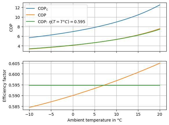
../_images/def76ffd6b1dbca75dbf26167bfcff217524ae8ebc9a839a535d02c8dfb9aef8.png — Fig. 8 Comparison of the COP of the heat pump calculated with a constant and a variable efficiency factor.#

From the graphs we can easily see, that the Carnot COP \(\text{COP}_\text{c}\) is (expectedly) higher than the actual COP. However, in the second subplot we see that the efficiency factor \(\eta\) is not constant.

There are two reasons for this. First, the definition of the Carnot COP in equation (eq. (4)) is not strictly correct. The effect of this is however only a minor one. The stronger effect is, that the thermodynamic losses (entropy production due to irreversibility) in each component are simply higher at lower temperature. We have prepared a separate section with the details on this phenomenon as a thermodynamic excursion here. This section will however not be part of the in-person workshop.

Preparing the results for the solph model#

To make these results usable for our solph model, we can simply export them to a .csv file:

export = results[["COP"]]
export.index.names = ["temperature"]
export.to_csv("COP-T-tespy.csv")