Part load performance in TESPy#
In this section we are investigating how operating the heat pump at part load affects the COP in the thermodynamic model. To do that, we will extend our model from the previous section to integrate the heat source and the heat sink air and water flow. Then we are investigating, how a specific design of the heat pump affects the operation at conditions different from that design state, i.e. when the ambient temperature changes, when the heat production changes and when both change simultaneously. The results are again fed back to the energy system optimization.
Tip
The TESPy documentation provides more information about part load modeling. There are some examples as well as a dedicated section in the documentation of the software’s modules: https://tespy.rtfd.io.
Introduction#
In TESPy it is possible to design a process and based on that design predict the part load operation of the overall system. To do that, component and process information are calculated from the design as a result and then remain unchanged in offdesign operation.
For example, the heat exchanger’s heat transfer coefficient can be calculated in the design based on the heat transferred and on the temperature levels at the two inlets and the two outlets of the component. Then for part load prediction, we can make the assumption that this value does not change (or it may follow a specific curve from a lookup table). This also means, that we reduce the degrees of freedom by one, for example the terminal temperature difference cannot be controlled anymore. It will be a result of changes in the flow regime at the heat exchanger and the assumptions concerning the heat transfer coefficient.
Note
A dedicated section in the excursion’s chapter will outline the effect of the single part load specifications we are providing in this example. You can find it here.
Preparing the model#
First we are going to prepare our TESPy model. To do that, we will slightly modify our topology according to the figure below. The overall specifications on heat exchanger temperature differences, compressor efficiency etc. will remain the unchanged.

Fig. 12 Component based thermodynamic model of the heat pump for part load modeling#
First, we import the HeatExchanger class to model the evaporator, the Condenser class to model the condenser
(instead of the SimpleHeatExchanger) we used in the first model, and finally the Source and Sink classes to
represent the ambient air in- and outlet as well as the heating system’s feed and return flow. We create instances of
the components and connect them according to the flowsheet.
from tespy.tools import logger


_ = logger.define_logging(screen_level=50)
from tespy.components import Condenser, HeatExchanger, CycleCloser, Compressor, Valve, Source, Sink
from tespy.connections import Connection, Ref
from tespy.networks import Network

wf = "R290"
nwk = Network(p_unit="bar", T_unit="C", iterinfo=False)

cp = Compressor("compressor")
ev = HeatExchanger("evaporator")
cd = Condenser("condenser")
va = Valve("expansion valve")
cc = CycleCloser("cycle closer")

so1 = Source("ambient air source")
si1 = Sink("ambient air sink")
so2 = Source("heating source")
si2 = Sink("heating sink")

c0 = Connection(va, "out1", cc, "in1", label="0")
c1 = Connection(cc, "out1", ev, "in2", label="1")
c2 = Connection(ev, "out2", cp, "in1", label="2")
c3 = Connection(cp, "out1", cd, "in1", label="3")
c4 = Connection(cd, "out1", va, "in1", label="4")

nwk.add_conns(c0, c1, c2, c3, c4)

c11 = Connection(so1, "out1", ev, "in1", label="11")
c12 = Connection(ev, "out1", si1, "in1", label="12")

c21 = Connection(so2, "out1", cd, "in2", label="21")
c22 = Connection(cd, "out2", si2, "in1", label="22")

nwk.add_conns(c11, c12, c21, c22)
Next step is parametrization again. Initially, we are going to skip the specification of the terminal temperature difference at the condenser due to numerical instability.
Tip
TESPy relies on good starting values for the solver. Since the applications you can model with the software are generic, it is impossible to provide starting values natively without knowing what is modeled. Generally, providing mass flow, pressure and enthalpy values lead to more stable convergence than providing, for example isentropic efficiency or terminal temperature differences. Also when changing working fluids, the convergence behavior may change completely. Therefore we provide a tutorial on how to build models with stable starting values on the TESPy documentation.
# connections
c2.set_attr(T=2)
c4.set_attr(T=40)

# components
Q_design = -9.1e3
cp.set_attr(eta_s=0.675)
cd.set_attr(Q=Q_design)

# connections
T_ambient_design = 7
c2.set_attr(fluid={wf: 1}, x=1.0)
c11.set_attr(fluid={"air": 1}, p=1.0, T=T_ambient_design)
c12.set_attr(T=Ref(c11, 1, -2))
c21.set_attr(fluid={"Water": 1}, p=3.0, T=30)
c22.set_attr(T=35)

# components
cd.set_attr(pr1=1, pr2=1)
ev.set_attr(pr1=1, pr2=1)

nwk.solve("design")
In the second step we finalize the specification values and rerun the simulation.
ev.set_attr(ttd_u=5)
c2.set_attr(T=None)

cd.set_attr(ttd_u=5)
c4.set_attr(T=None)

nwk.solve("design")

nwk.print_results(colored=False)
nwk.save("design-state")
nwk.save("tmp")

nwk.results["Connection"]
##### RESULTS (Compressor) #####
+------------+----------+----------+----------+--------+
|            |        P |    eta_s |       pr |   igva |
|------------+----------+----------+----------+--------|
| compressor | 1.86e+03 | 6.75e-01 | 2.72e+00 |    nan |
+------------+----------+----------+----------+--------+
##### RESULTS (HeatExchanger) #####
+------------+-----------+----------+----------+----------+----------+----------+----------+----------+----------+
|            |         Q |       kA |   td_log |    ttd_u |    ttd_l |      pr1 |      pr2 |    zeta1 |    zeta2 |
|------------+-----------+----------+----------+----------+----------+----------+----------+----------+----------|
| evaporator | -7.24e+03 | 1.85e+03 | 3.92e+00 | 5.00e+00 | 3.00e+00 | 1.00e+00 | 1.00e+00 | 0.00e+00 | 0.00e+00 |
+------------+-----------+----------+----------+----------+----------+----------+----------+----------+----------+
##### RESULTS (CycleCloser) #####
+--------------+------------------+-------------------+
|              |   mass_deviation |   fluid_deviation |
|--------------+------------------+-------------------|
| cycle closer |         0.00e+00 |          0.00e+00 |
+--------------+------------------+-------------------+
##### RESULTS (Valve) #####
+-----------------+----------+----------+
|                 |       pr |     zeta |
|-----------------+----------+----------|
| expansion valve | 3.68e-01 | 1.04e+11 |
+-----------------+----------+----------+
##### RESULTS (Condenser) #####
+-----------+-----------+----------+----------+----------+----------+----------+----------+----------+----------+
|           |         Q |       kA |   td_log |    ttd_u |    ttd_l |      pr1 |      pr2 |    zeta1 |    zeta2 |
|-----------+-----------+----------+----------+----------+----------+----------+----------+----------+----------|
| condenser | -9.10e+03 | 1.26e+03 | 7.21e+00 | 5.00e+00 | 1.00e+01 | 1.00e+00 | 1.00e+00 | 0.00e+00 | 0.00e+00 |
+-----------+-----------+----------+----------+----------+----------+----------+----------+----------+----------+
##### RESULTS (Connection) #####
+----+-----------+-----------+-----------+-----------+
|    |         m |         p |         h |         T |
|----+-----------+-----------+-----------+-----------|
|  0 | 2.683e-02 | 5.041e+00 | 3.071e+05 | 2.000e+00 |
|  1 | 2.683e-02 | 5.041e+00 | 3.071e+05 | 2.000e+00 |
|  2 | 2.683e-02 | 5.041e+00 | 5.771e+05 | 2.000e+00 |
|  3 | 2.683e-02 | 1.369e+01 | 6.463e+05 | 5.453e+01 |
|  4 | 2.683e-02 | 1.369e+01 | 3.071e+05 | 4.000e+01 |
| 11 | 3.601e+00 | 1.000e+00 | 4.063e+05 | 7.000e+00 |
| 12 | 3.601e+00 | 1.000e+00 | 4.043e+05 | 5.000e+00 |
| 21 | 4.355e-01 | 3.000e+00 | 1.260e+05 | 3.000e+01 |
| 22 | 4.355e-01 | 3.000e+00 | 1.469e+05 | 3.500e+01 |
+----+-----------+-----------+-----------+-----------+
| m | m_unit | v | v_unit | p | p_unit | h | h_unit | T | T_unit | ... | Td_bp_unit | vol | vol_unit | x | x_unit | s | s_unit | Water | air | R290 | |
|---|---|---|---|---|---|---|---|---|---|---|---|---|---|---|---|---|---|---|---|---|---|
| 0 | 0.026834 | kg / s | 0.000708 | m3 / s | 5.040999 | bar | 307147.999598 | J / kg | 2.000000 | C | ... | C | 0.026391 | m3 / kg | 0.274511 | - | 1389.278120 | J / kgK | NaN | NaN | 1.0 |
| 1 | 0.026834 | kg / s | 0.000708 | m3 / s | 5.040999 | bar | 307147.999598 | J / kg | 2.000000 | C | ... | C | 0.026391 | m3 / kg | 0.274511 | - | 1389.278120 | J / kgK | NaN | NaN | 1.0 |
| 2 | 0.026834 | kg / s | 0.002445 | m3 / s | 5.040999 | bar | 577063.427393 | J / kg | 2.000000 | C | ... | C | 0.091112 | m3 / kg | 1.000000 | - | 2370.253689 | J / kgK | NaN | NaN | 1.0 |
| 3 | 0.026834 | kg / s | 0.000981 | m3 / s | 13.694204 | bar | 646266.316995 | J / kg | 54.530607 | C | ... | C | 0.036554 | m3 / kg | -1.000000 | - | 2439.993233 | J / kgK | NaN | NaN | 1.0 |
| 4 | 0.026834 | kg / s | 0.000057 | m3 / s | 13.694204 | bar | 307147.999598 | J / kg | 40.000000 | C | ... | C | 0.002139 | m3 / kg | 0.000000 | - | 1359.354602 | J / kgK | NaN | NaN | 1.0 |
| 11 | 3.600738 | kg / s | 2.894125 | m3 / s | 1.000000 | bar | 406330.818533 | J / kg | 7.000000 | C | ... | C | 0.803759 | m3 / kg | -1.000000 | - | 3821.630622 | J / kgK | NaN | 1.0 | NaN |
| 12 | 3.600738 | kg / s | 2.873397 | m3 / s | 1.000000 | bar | 404319.289111 | J / kg | 5.000000 | C | ... | C | 0.798002 | m3 / kg | -1.000000 | - | 3814.424683 | J / kgK | NaN | 1.0 | NaN |
| 21 | 0.435516 | kg / s | 0.000437 | m3 / s | 3.000000 | bar | 126003.690096 | J / kg | 30.000000 | C | ... | C | 0.001004 | m3 / kg | -1.000000 | - | 436.664733 | J / kgK | 1.0 | NaN | NaN |
| 22 | 0.435516 | kg / s | 0.000438 | m3 / s | 3.000000 | bar | 146898.420887 | J / kg | 35.000000 | C | ... | C | 0.001006 | m3 / kg | -1.000000 | - | 505.027895 | J / kgK | 1.0 | NaN | NaN |
9 rows × 21 columns
Design Mode#
Now we are going to investigate, how the COP of the heat pump changes, when changing the ambient temperature and the heat demand. For this two steps will be taken:
Modification of temperature and heat without changing any of the component specifications. That means, e.g. that the compressor’s efficiency or the heat exchangers’ temperature differences will stay constant.
Modification of temperature and heat while applying part load assumptions for the compressor and the heat exchangers. These are implemented with lookup tables, where the change of mass flow through the component leads to a change in efficiency or temperature difference.
Influence of the ambient temperature#
First, we investigate the influence of the ambient temperature. We have done this in the first TESPy section already, see Simple TESPy heat pump model, but since we change the topology we repeat this step.
import numpy as np
import pandas as pd
from matplotlib import pyplot as plt


temperature_range = np.arange(-10, 21)
results_temperature = pd.DataFrame(
    index=temperature_range,
    columns=["compressor-power", "pressure-ratio", "COP"]
)

for temperature in temperature_range:

    c11.set_attr(T=temperature)
    nwk.solve("design")

    results_temperature.loc[temperature, "compressor-power"] = cp.P.val
    results_temperature.loc[temperature, "pressure-ratio"] = cp.pr.val
    results_temperature.loc[temperature, "COP"] = abs(cd.Q.val) / cp.P.val
We create three subplots for the results: Compressor power \(\dot W_\text{cp}\), the compressor pressure ratio and COP over the ambient temperature level. We can see the same trend in Fig. 13 as we saw in the previous section in Fig. 8.
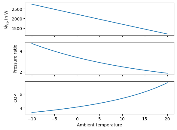
Fig. 13 Influence of the ambient temperature on the compressor power, its pressure ratio and the COP without modeling part load behavior.#
fig, ax = plt.subplots(3, sharex=True)

ax[0].plot(temperature_range, results_temperature["compressor-power"])
ax[1].plot(temperature_range, results_temperature["pressure-ratio"])
ax[2].plot(temperature_range, results_temperature["COP"])

ax[0].set_ylabel("$\dot W_\\mathrm{cp}$ in W")
ax[1].set_ylabel("Pressure ratio")
ax[2].set_ylabel("COP")
_ = ax[2].set_xlabel("Ambient temperature")

plt.close()
Influence of the heat production#
Second, we investigate the influence of the heat production. We can define a heat range relative to the design heat production spanning from 50 % to 100 % load. The ambient temperature is reset back to the previous state, and we can loop over the part load values.
Note
The compressor of a heat pump will be the component restricting lower and upper operational limits. Using 50 % heat production as minumum value scales to about 50 % compressor load. The value is an assumption we make for this tutorial. In the best case, you can retrieve exact data from a manufacturer.
heat_range = np.linspace(0.5, 1.0, 11) * Q_design
results_heat = pd.DataFrame(
    index=heat_range,
    columns=["compressor-power", "pressure-ratio", "COP"]
)
c11.set_attr(T=T_ambient_design)

for heat in heat_range[::-1]:
    cd.set_attr(Q=heat)
    nwk.solve("design")

    results_heat.loc[heat, "compressor-power"] = cp.P.val
    results_heat.loc[heat, "pressure-ratio"] = cp.pr.val
    results_heat.loc[heat, "COP"] = abs(cd.Q.val) / cp.P.val
Again we create a plot with the influence of the heat production on the compressor’s parameters and on the COP in Fig. 14. It becomes obvious that neither the compressor’s pressure ratio nor the COP are affected by the changing heat load. Only the compressor power requirement scales with the load. The reason for this is, that the compressor’s efficiency and the temperature differences (and therefore the evaporation and condensation temperatures) do not change with changing load due to our model specifications.
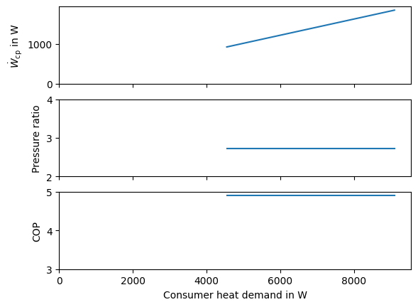
Fig. 14 Influence of the heat load on the compressor power, its pressure ratio and the COP without modeling part load behavior.#
fig, ax = plt.subplots(3, sharex=True)

ax[0].plot(np.abs(heat_range), results_heat["compressor-power"])
ax[1].plot(np.abs(heat_range), results_heat["pressure-ratio"])
ax[2].plot(np.abs(heat_range), results_heat["COP"])

ax[0].set_ylabel("$\dot W_\\mathrm{cp}$ in W")
ax[1].set_ylabel("Pressure ratio")
ax[2].set_ylabel("COP")

ax[0].set_ylim([0, results_heat["compressor-power"].max() * 1.05])
ax[1].set_ylim([2, 4])
ax[2].set_ylim([3, 5])
ax[2].set_xlim([0, np.abs(heat_range).max() * 1.05])

ax[2].set_xlabel("Consumer heat demand in W")

plt.close()
Part load simulation#
The assumptions made in the previous section are not really reasonable: A heat exchanger cannot always hold the temperature difference independent of the (changing) flow regimes, when it has been constructed for a specific operational point. The same applies for the compressor: We can expect that the efficiency changes when it is not operated in optimal conditions. Therefore, this sections shows how we can make assumptions on the part load behavior of these components.
Influence of the ambient temperature#
First, we are going to investigate the ambient temperature influence. To do this, instead of using the "design" mode
for our simulation we are using the "offdesign" mode. The offdesign mode can access a design specification and based
on that and the current operational point predict part load efficiencies.
For the components that means, that the compressor’s efficiency will not be an input parameter anymore, but a
characteristic curve will be applied instead. The characteristic holds a lookup table connecting the change of mass flow
relative to the design point mass flow with the change in efficiency. For the evaporator and the condenser we make
similar assumptions: Instead of having constant temperature difference values, the heat transfer coefficient kA is
applied together with a characteristic curve, modifying its value depending on the change of mass flows relative to the
design point mass flows.
Caution
The default characteristic lines in TESPy are very generic, do NOT consider them as written in stone!
They may not represent components from specific manufacturers in the appropriate way. It is also possible to derive characteristics from measurement data. To implement your custom characteristic lines see the respective sections in the TESPy online documentation.
In our setup we allow extrapolation on the compressor characteristic line, and we run the same loop over the temperature as we had in the first analysis.
cd.set_attr(Q=Q_design)
cp.set_attr(design=["eta_s"], offdesign=["eta_s_char"])
cp.eta_s_char.char_func.extrapolate = True
ev.set_attr(design=["ttd_u"], offdesign=["kA_char"])
cd.set_attr(design=["ttd_u"], offdesign=["kA_char"])

results_temperature_partload = pd.DataFrame(
    index=temperature_range,
    columns=["compressor-power", "pressure-ratio", "COP"]
)


for temperature in temperature_range:

    c11.set_attr(T=temperature)
    nwk.solve("offdesign", design_path="design-state")

    results_temperature_partload.loc[temperature, "compressor-power"] = cp.P.val
    results_temperature_partload.loc[temperature, "pressure-ratio"] = cp.pr.val
    results_temperature_partload.loc[temperature, "COP"] = abs(cd.Q.val) / cp.P.val
We make the same plots as before, comparing the results of the design point calculations with those that take part-load into account. The Fig. 15 shows the comparison of both approaches. The last subplot is the deviation in COP, which is at an overall low level. Only for very high ambient temperature levels, which are nearly at the heat supply temperature level the deviation increases to about 5 % with respect to the model accounting for part load behavior.
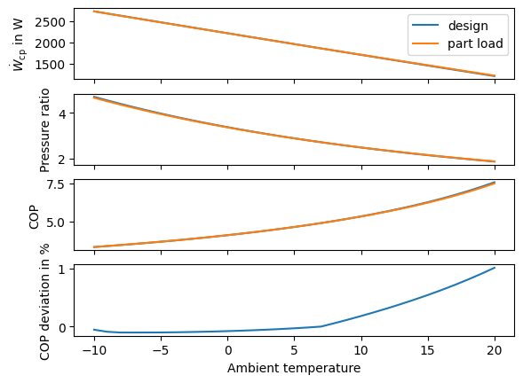
Fig. 15 Influence of the ambient temperature on the compressor power, its pressure ratio and the COP when considering part load behavior.#
fig, ax = plt.subplots(4, sharex=True)

ax[0].plot(temperature_range, results_temperature["compressor-power"], label="design")
ax[1].plot(temperature_range, results_temperature["pressure-ratio"])
ax[2].plot(temperature_range, results_temperature["COP"])

ax[0].plot(temperature_range, results_temperature_partload["compressor-power"], label="part load")
ax[1].plot(temperature_range, results_temperature_partload["pressure-ratio"])
ax[2].plot(temperature_range, results_temperature_partload["COP"])

ax[3].plot(temperature_range, (results_temperature["COP"] - results_temperature_partload["COP"]) / results_temperature_partload["COP"] * 100)

ax[0].set_ylabel("$\dot W_\\mathrm{cp}$ in W")
ax[1].set_ylabel("Pressure ratio")
ax[2].set_ylabel("COP")
ax[3].set_ylabel("COP deviation in %")

ax[0].legend()

_ = ax[3].set_xlabel("Ambient temperature")

plt.close()
Note
A way of controlling whether your setup for the part load modeling is correct is to check if offdesign parameter settings of the model lead to the same result as in the design parameter specifications. If these numbers do not align, there might be something wrong the model setup. In this case, we always have the design heat load and we have to compare the results at the design ambient temperature, i.e. 2 °C.
results_temperature.loc[T_ambient_design]
compressor-power    1857.010557
pressure-ratio         2.716565
COP                    4.900349
Name: 7, dtype: object
results_temperature_partload.loc[T_ambient_design]
compressor-power    1857.010557
pressure-ratio         2.716565
COP                    4.900349
Name: 7, dtype: object
Influence of the heat production#
Next we are checking the influence of the heat production of the heat pump on our COP. We reset the temperature back to the ambient design temperature value and rerun the offdesign simulations with the heat range specified earlier.
c11.set_attr(T=T_ambient_design)
results_heat_partload = pd.DataFrame(
    index=heat_range,
    columns=["compressor-power", "pressure-ratio", "COP"]
)

for heat in heat_range[::-1]:
    cd.set_attr(Q=heat)
    nwk.solve("offdesign", design_path="design-state")

    results_heat_partload.loc[heat, "compressor-power"] = cp.P.val
    results_heat_partload.loc[heat, "pressure-ratio"] = cp.pr.val
    results_heat_partload.loc[heat, "COP"] = abs(cd.Q.val) / cp.P.val
Again we plot our results against the results of the simulation in design mode (Fig. 16). The COP of both simulations matches quite well for all heat loads above 75 % of design heat production. For lower heat production values the part load considering simulations show lower COP than the design simulation. When looking at the compressor’s pressure ratio its value decreases with decreasing heat load. This seems odd at first, because a lower pressure ratio would indicate lower compressor power. The reason for the increasing compressor power demand is to be sought in its part load efficiency, which decreases faster than the pressure ratio.
Tip
A detailed analysis of the influence factors on the heat pump’s performance in part load simulation is provided in this excursion.
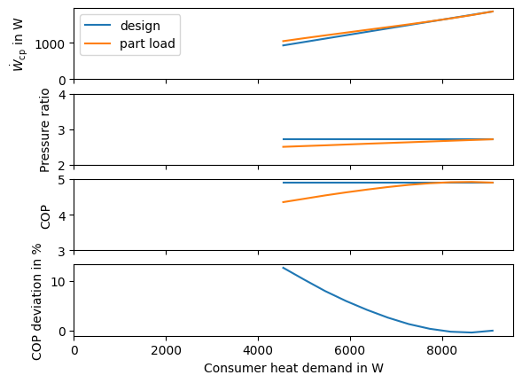
Fig. 16 Influence of the heat load on the compressor power, its pressure ratio and the COP when considering part load behavior.#
fig, ax = plt.subplots(4, sharex=True)

ax[0].plot(np.abs(heat_range), results_heat["compressor-power"], label="design")
ax[1].plot(np.abs(heat_range), results_heat["pressure-ratio"])
ax[2].plot(np.abs(heat_range), results_heat["COP"])
ax[0].plot(np.abs(heat_range), results_heat_partload["compressor-power"], label="part load")
ax[1].plot(np.abs(heat_range), results_heat_partload["pressure-ratio"])
ax[2].plot(np.abs(heat_range), results_heat_partload["COP"])

ax[3].plot(np.abs(heat_range), (results_heat["COP"] - results_heat_partload["COP"]) / results_heat_partload["COP"] * 100)

ax[0].set_ylabel("$\dot W_\\mathrm{cp}$ in W")
ax[1].set_ylabel("Pressure ratio")
ax[2].set_ylabel("COP")
ax[3].set_ylabel("COP deviation in %")

ax[0].set_ylim([0, results_heat["compressor-power"].max() * 1.05])
ax[1].set_ylim([2, 4])
ax[2].set_ylim([3, 5])
ax[3].set_xlim([0, np.abs(heat_range).max() * 1.05])

ax[0].legend()

_ = ax[3].set_xlabel("Consumer heat demand in W")

plt.close()
We can have the same look at the results from the dataframes. Since we inspected the part load behavior for the heat
output at the design temperature level of the ambient, we should see equal values in the results for the design heat
production, i.e. -10,000.0 W.
results_heat_partload.loc[Q_design]
compressor-power    1857.010557
pressure-ratio         2.716565
COP                    4.900349
Name: -9100.0, dtype: object
results_heat.loc[Q_design]
compressor-power    1857.010557
pressure-ratio         2.716565
COP                    4.900349
Name: -9100.0, dtype: object
Variable temperature and heat production#
Now we want to combine both influence factors. We can do that by looping over the ambient temperature and the heat load simultaneously. Since our input data for the energy system optimization are based on the ambient temperature, we investigate the influence of the heat load per temperature value.
temperature_range = np.arange(-10, 21)

results = {}


for temperature in temperature_range:
    results[temperature] = pd.DataFrame(index=heat_range, columns=["COP", "compressor-power", "T-evaporation", "T-condensation"])
    c11.set_attr(T=temperature)
    for heat in heat_range[::-1]:
        cd.set_attr(Q=heat)
        if heat == heat_range[-1]:
            nwk.solve("offdesign", design_path="design-state", init_path="tmp")
            nwk.save("tmp")
        else:
            nwk.solve("offdesign", design_path="design-state")

        results[temperature].loc[heat, "COP"] = abs(cd.Q.val) / cp.P.val
        results[temperature].loc[heat, "compressor-power"] = cp.P.val
        results[temperature].loc[heat, "T-evaporation"] = c2.T.val
        results[temperature].loc[heat, "T-condensation"] = c4.T.val
We can plot some results, e.g. for every 10th temperature value in Fig. 17. These
results can then be transferred to the oemof-solph simulation.
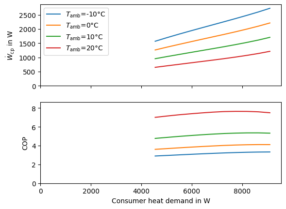
Fig. 17 Influence of the ambienht temperature and heat load on the compressor power and the COP when considering part load behavior.#
power_max = 0
COP_max = 0

fig, ax = plt.subplots(2, sharex=True)

for temp in temperature_range[::10]:

    ax[0].plot(np.abs(results[temp].index), results[temp]["compressor-power"], label="$T_\\mathrm{amb}$=" + str(temp) + "°C")
    ax[1].plot(np.abs(results[temp].index), results[temp]["COP"])
    COP_max = max(results[temp]["COP"].max(), COP_max)
    power_max = max(results[temp]["compressor-power"].max(), power_max)

ax[0].legend()
ax[0].set_ylabel("$\dot W_\\mathrm{cp}$ in W")
ax[0].set_ylim([0, power_max * 1.05])
ax[1].set_ylabel("COP")
ax[1].set_ylim([0, COP_max + 1])
ax[1].set_xlim([0, np.abs(heat_range).max() * 1.05])
_ = ax[1].set_xlabel("Consumer heat demand in W")

plt.close()
Preparing the data for oemof-solph#
To prepare the data for the usage in the mixed integer linear model, we have to linearize the outcomes of our simulation. To do that, we can use a simple least squares method from the numpy package [9], [10]. The least squares will give us the slope and the y-axis offset, both of which are required in the mixed integer model.
def least_squares(x, y):
    A = np.vstack([x, np.ones(len(x))]).T
    slope, offset = np.linalg.lstsq(A, y, rcond=None)[0]
    return slope, offset
In Fig. 18 we can make a plot to look at the deviation between the assumption of a constant efficiency value (as in the first attempt in this section), the linearized variant and the actual simulation. For example, we can have a look at the design conditions for the ambient temperature. We can see that the deviation between the linearized model and the actual simulation is below 1.5 % for all heat load values. The assumption of a constant efficiency factor leads to a high deviation especially with lower heat production up to 18 %.
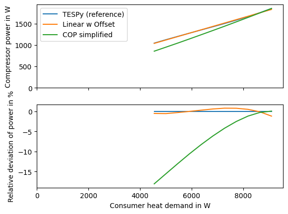
Fig. 18 Comparison of the compressor power depending on the heat pump’s heat load for the simplified approach and in the part load simulation.#
Furthermore, we can plot the linearization of a selected amount of simulation points in Fig. 19. We can see, that both, offset and slope, change for every ambient temperature value.
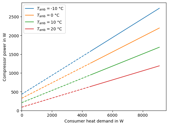
Fig. 19 Linearized compressor power to heat load.#
x = -results[T_ambient_design].index.values.astype(float)
y = results[T_ambient_design]["compressor-power"].values.astype(float)
yy_tespy = y


COP_c_simple = (
    (results[T_ambient_design]["T-condensation"] + 273.15) /
    (results[T_ambient_design]["T-condensation"] - results[T_ambient_design]["T-evaporation"])
)
eta_c_simple = 0.5945

fig, ax = plt.subplots(2, sharex=True)

ax[0].plot(x, yy_tespy, label="TESPy (reference)")

slope, offset = least_squares(x, y)
yy_offset = offset + slope * x
ax[0].plot(x, yy_offset, label="Linear w Offset")
ax[0].plot(x, x / (COP_c_simple * eta_c_simple), label="COP simplified")

ax[1].plot(x, (yy_tespy - yy_tespy) / yy_tespy * 100)
ax[1].plot(x, (yy_offset - yy_tespy) / yy_tespy * 100)
ax[1].plot(x, (x / (COP_c_simple * eta_c_simple) - yy_tespy) / yy_tespy * 100)

ax[0].legend()
ax[0].set_ylabel("Compressor power in W")
ax[0].set_ylim([0, y.max() * 1.05])
ax[1].set_ylabel("Relative deviation of power in %")
ax[1].set_xlim([0, x.max() * 1.05])
_ = ax[1].set_xlabel("Consumer heat demand in W")

plt.close()
fig, ax = plt.subplots(1)

for temp in temperature_range[::10]:

    x = -results[temp].index.values.astype(float)
    y = results[temp]["compressor-power"].values.astype(float)
    slope, offset = least_squares(x, y)
    p = ax.plot(x, slope * x + offset, label="$T_\\mathrm{amb}=$" + str(temp) + " °C")  # get line information to extract color
    ax.plot([0, x.min()], slope * np.array([0, x.min()]) + offset, "--", color=p[0].get_color())
    power_max = max(results[temp]["compressor-power"].max(), power_max)

ax.set_ylim([0, power_max * 1.05])
ax.set_ylabel("Compressor power in W")
ax.set_xlim([0, x.max() * 1.05])
ax.legend()
_ = ax.set_xlabel("Consumer heat demand in W")

plt.close()
The final step is to export the data for the OffsetConverter of oemof-solph.
oemof-solph expects a conversion factor and the normed offset per ambient temperature level for the input and
output flows except a single reference flow. The reference flow will be the heat output of the heat pump. Therefore,
we need to calculate the electricity conversion factor and normed offset as a function of the heat output with the
least_squares function, dump the results into a new DataFrame and export to csv.
Caution
oemof-solph expects a normed offset, that is the offset value divided by the rated heat output.
export_df = pd.DataFrame(index=temperature_range, columns=["slope", "offset"])

for key, data in results.items():
    x = -data.index.values.astype(float)
    y = data["compressor-power"].values.astype(float)
    export_df.loc[key] = least_squares(x, y)

export_df["offset"] /= -Q_design
export_df.to_csv("coefficients-offset-converter.csv")