Entropy Analysis of the COP

Introduction

Strictly speaking the definition of the Carnot COP of a heat pump following eq. (4) is only valid for a process, that consists of two isentropic subprocesses (compression and expansion) and two isothermal subprocesses (evaporation and condensation). For this to be possible, the heat pump would need to use a turbine instead of an expansion valve and the fluid must be in the two-phase region again after the compression. While compression of dry working fluids (the isentropics reach back into the saturation dome at higher pressures) is technically possible, expanding saturated liquid is technically not feasible. Still, we can apply the Carnot method to investigate our heat pump cycle from thermodynamically, but we have to make some changes. However, this even allows us to show the contribution of the individual components in the cycle to its thermodynamic “non-optimality”.[1]

Carnot COP

However, we can slightly adapt the COP definition from eq. (4) by replacing the temperature levels \(T_\text{max}\) and \(T_\text{min}\), with the thermodynamic mean temperature of the heat production \(T_\text{m,prod}\) and the heat consumption \(T_\text{m,cons}\) in eq. (11). The thermodynamic mean temperature is defined by eq. (12).

(11)\[ \text{COP}_\text{c} = \frac{T_\mathrm{m,prod}}{T_\mathrm{m,prod} - T_\mathrm{m,cons}}\]

(12)\[ T_\text{m,Q} = \frac{\dot Q}{\dot S_\text{Q}}\]

With this, it is possible to calculate the Carnot COP with the TESPy model by calling the entropy balance equations on the components to obtain the thermodynamic mean temperature of the condensation and evaporation.

Note

The entropy analysis feature is still to be completed. If anybody is interested in contributing on this topic, please reach out to the developers via the TESPy github repository. Your contribution is highly appreciated!

The simple_heat_pump function imported in this section lies in a separate python document. You can download it: heat_pump_models.py.

from heat_pump_models import simple_heat_pump


import pandas as pd
import numpy as np
from matplotlib import pyplot as plt


def carnot_COP_temperature_variation(nwk, temperature_range):

    results = pd.DataFrame(
        index=temperature_range,
        columns=["COP", "COP_carnot", "COP_carnot_simple"]
    )

    c2, c4 = nwk.get_conn(["2", "4"])
    ev, cd, cp, va = nwk.get_comp(
        ["evaporator", "condenser", "compressor", "expansion valve"]
    )

    for T in temperature_range:
        c2.set_attr(T=T)
        nwk.solve("design")
        for component in [ev, cd, cp, va]:
            component.entropy_balance()

        results.loc[T, "COP"] = abs(cd.Q.val) / cp.P.val
        results.loc[T, "COP_carnot"] = cd.T_mQ / (cd.T_mQ - ev.T_mQ)
        results.loc[T, "COP_carnot_simple"] = (
            c4.T.val_SI / (c4.T.val - c2.T.val)
        )


    results["deviation"] = results["COP_carnot"] / results["COP_carnot_simple"]

    return results


nwk = simple_heat_pump("R290")
temperature_range = np.linspace(-10, 31, 32)
results = carnot_COP_temperature_variation(nwk, temperature_range)


fig, ax = plt.subplots(2, sharex=True)

label = "$\mathrm{COP}_\mathrm{c,simple}$"
ax[0].plot(temperature_range, results["COP_carnot_simple"], label=label)
label = "$\mathrm{COP}_\mathrm{c}$"
ax[0].plot(temperature_range, results["COP_carnot"], label=label)
ax[0].plot(temperature_range, results["COP"], label="$\mathrm{COP}$")
ax[0].set_ylabel("COP")
ax[0].legend()

label = "$\\frac{\mathrm{COP}_\mathrm{c}}{\mathrm{COP}_\mathrm{c,simple}}$"
ax[1].plot(temperature_range, results["deviation"], label=label)
ax[1].set_ylabel("COP ratio")
ax[1].legend()

ax[1].set_xlabel("Evaporation temperature in °C")

_ = [_.grid() for _ in ax]
_ = [_.set_axisbelow(True) for _ in ax]

plt.close()

FutureWarning: The API for the component HeatExchangerSimple will change with the next major release, please import SimpleHeatExchanger instead.

We can observe, that there is a difference between the two approaches in Fig. 22, however it does not explain, the sharp increase in the efficiency factor as seen in Fig. 8. To explain that phenomenon, we have to disect the calculation of the COP of the heat pump a further.

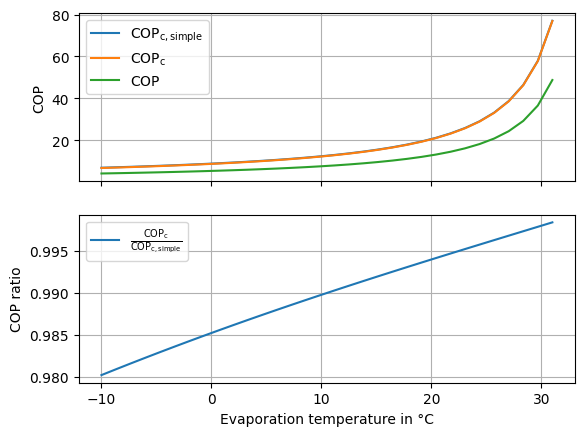
Fig. 22 Comparison of the carnot COP calcualted with the simplified method and the exact method.

Irreversibility Production

To do that, we can first reorder the definition of the COP in the following equation:

(13)\[\begin{split}\begin{align} \text{COP} = & \frac{|\dot Q_\text{prod}|}{\dot W}\\ = & \frac{|\dot Q_\text{prod}|}{|\dot Q_\text{prod}| - \dot Q_\text{cons}}\\ = & \frac{1}{\frac{|\dot Q_\text{prod}| - \dot Q_\text{cons}}{|\dot Q_\text{prod}|}}\\ = & \frac{1}{1 - \frac{\dot Q_\text{cons}}{|\dot Q_\text{prod}|}} \end{align}\end{split}\]

Then with the definition of the thermodynamic mean temperature, we can replace the heat transfers.

(14)\[ \text{COP} = \frac{1}{1 - \frac{T_\text{m,cons} \cdot \dot S_\text{q,cons}}{T_\text{m,prod} \cdot |\dot S_\text{q,prod}|}}\]

Finally, the second law of thermodynamics allows us to replace the entropy transferred to the system from the evaporator \(\dot S_\text{q,cons}\) with difference between the entropy transferred to the heat consumer \(\dot S_\text{q,prod}\) and all entropy production inside the thermodynamic cycle \(\sum \dot S_{\text{irr,}i}\).

(15)\[ \dot S_\text{q,cons} = |\dot S_\text{q,prod}| - \sum \dot S_{\text{irr,}i}\]

We make further simplifications of the expression below the line in eq. (14).

(16)\[\begin{split}\begin{align} \frac{T_\text{m,cons} \cdot \dot S_\text{q,cons}}{T_\text{m,prod} \cdot |\dot S_\text{q,prod}|} = & \frac{T_\text{m,cons}}{T_\text{m,prod}} \cdot \frac{|\dot S_\text{q,prod}| - \sum \dot S_{\text{irr,}i}}{|\dot S_\text{q,prod}|} \\ = & \frac{T_\text{m,cons}}{T_\text{m,prod}} \cdot \left(1 - \frac{\sum \dot S_{\text{irr,}i}}{|\dot S_\text{q,prod}|}\right) \\ = & \frac{T_\text{m,cons}}{T_\text{m,prod}} - \frac{T_\text{m,cons} \cdot \sum \dot S_{\text{irr,}i}}{T_\text{m,prod} \cdot |\dot S_\text{q,prod}|} \\ = & \frac{T_\text{m,cons}}{T_\text{m,prod}} - \frac{T_\text{m,cons} \cdot \sum \dot S_{\text{irr,}i}}{|\dot Q_\text{m,prod}|} \end{align}\end{split}\]

Finally, we obtain a formula for the COP, where the first term is identical to the inverse value of the Carnot COP and the second part are the thermodynamic losses induced by the individual components. We can see that the higher the evaporation temperature level is, the higher the thermodynamic inefficiencies of the individual components are the lower the COP or - at a given Carnot COP - the lower the efficiency factor is.

(17)\[ \text{COP} = \frac{1}{1 - \frac{T_\text{m,cons}}{T_\text{m,prod}} + \sum \dot S_{\text{irr,}i} \cdot \frac{T_\text{m,cons}}{\dot Q_\text{prod}}}\]

With this information we can extend our method to calculate the COP of the heat pump accordingly.

def entropy_analysis_temperature_variation(nwk, temperature_range):

    c2, c4 = nwk.get_conn(["2", "4"])
    ev, cd, cp, va = nwk.get_comp(
        ["evaporator", "condenser", "compressor", "expansion valve"]
    )
    component_list = [ev, cd, cp, va]

    results = pd.DataFrame(
        index=temperature_range,
        columns=[
            "COP", "COP_carnot", "COP_carnot_simple",
            "T_m,ev", "T_m,cd"
        ] + [f"S_irr,{component.label}" for component in component_list]
    )

    for T in temperature_range:
        c2.set_attr(T=T)
        nwk.solve("design")
        for component in component_list:
            component.entropy_balance()
            results.loc[T, f"S_irr,{component.label}"] = component.S_irr

        results.loc[T, "T_m,ev"] = ev.T_mQ
        results.loc[T, "T_m,cd"] = cd.T_mQ
        results.loc[T, "COP"] = abs(cd.Q.val) / cp.P.val
        results.loc[T, "COP_carnot"] = cd.T_mQ / (cd.T_mQ - ev.T_mQ)
        results.loc[T, "COP_carnot_simple"] = (
            c4.T.val_SI / (c4.T.val - c2.T.val)
        )
        results.loc[T, "Q_condenser"] = abs(cd.Q.val)


    results["deviation"] = results["COP_carnot"] / results["COP_carnot_simple"]

    return results

Then, we can investigate the temperature dependency of all relevant influence factors.

temperature_range = np.linspace(-10, 31, 32)
results = entropy_analysis_temperature_variation(nwk, temperature_range)

fig, ax = plt.subplots(1)

label = "$\mathrm{COP}_\mathrm{c}$"
ax.plot(temperature_range, results["COP_carnot"], label=label)
ax.plot(temperature_range, results["COP"], label="$\mathrm{COP}$")
ax.plot(
    temperature_range,
    1 / (
        1 / results["COP_carnot"]
        + (
            results["S_irr,compressor"] + results["S_irr,expansion valve"]
        ) * results["T_m,ev"]
        / results["Q_condenser"]
    ),
    "x", label="$\mathrm{COP}_\mathrm{entropy method}$"
)
ax.set_ylabel("COP")
ax.legend()

ax.grid()
ax.set_axisbelow(True)
plt.close()

fig, ax = plt.subplots(2, sharex=True)

ax[0].plot(temperature_range, results["S_irr,compressor"], label="compressor")
ax[0].plot(temperature_range, results["S_irr,expansion valve"], label="expansion valve")
ax[0].plot(temperature_range, results["S_irr,compressor"] + results["S_irr,expansion valve"], label="total")
ax[0].set_ylabel("$\dot S_\mathrm{irr}$")
ax[0].legend()

ax[1].plot(temperature_range, results["S_irr,compressor"] * results["T_m,ev"] / results["Q_condenser"], label="compressor")
ax[1].plot(temperature_range, results["S_irr,expansion valve"] * results["T_m,ev"] / results["Q_condenser"], label="expansion valve")
ax[1].plot(temperature_range, (results["S_irr,compressor"] + results["S_irr,expansion valve"]) * results["T_m,ev"] / results["Q_condenser"], label="total")
ax[1].set_ylabel("$\\frac{\dot S_\mathrm{irr} \cdot T_\mathrm{m,ev}}{\dot Q_\mathrm{cd}}$")
ax[1].set_xlabel("Evaporation temperature in °C")

_ = [_.grid() for _ in ax]
_ = [_.set_axisbelow(True) for _ in ax]

plt.close()

First, we can show, that the COP calculated with the entropy method retrieves the same result as the COP retrieved from the standard calculation in Fig. 23. Then we can inspect the dependency of the irreversibility elements in Fig. 24. Here we can see, that the decline of irreversibility production with increasing evaporation temperature is steeper that the increase of the evaporation temperature. That is the reason, we have an increasing efficiency factor when the evaporation temperature level rises.

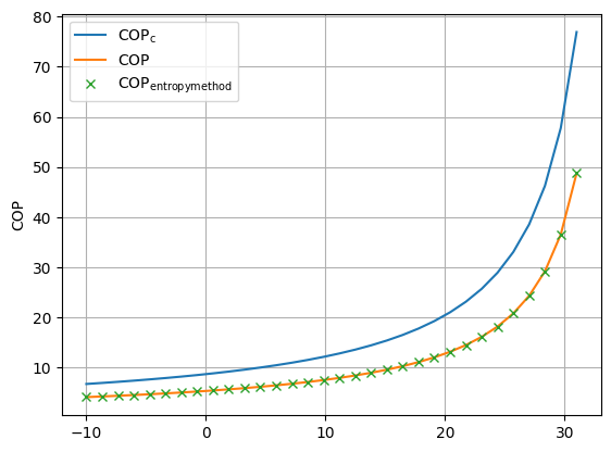
Fig. 23 Validation of the entropy method for the calculation of the heat pump’s COP.

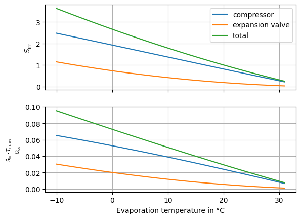
Fig. 24 Comparison of the effects of the different irreversibility elements.

Investigating Working Fluids

Finally, we can make an investigation for different types of working fluids, as the efficiency factor not only depends on the temperature level of evaporation, but also on the fluid itself. As examples, we assess working fluids from the different classifications (for more information see e.g. [11, 12, 13, 14]), which are roughly defined by the slope of the dew line in the Ts-diagram, i.e.

• wet: It has a forwards-facing slope

• isentropic: It is vertical (parallel to the isentropics)

• dry: It has a backwards-facing slope

from CoolProp.CoolProp import PropsSI as PSI


fluids = {
    "Propane": {
        "classification": "isentropic",
        "color": "tab:blue"
    },
    "Pentane": {
        "classification": "dry",
        "color": "tab:red"
    },
    "Ammonia": {
        "classification": "wet",
        "color": "tab:green"
    }
}
colors = []
saturation_domes = {fluid: {} for fluid in fluids}

fig, ax = plt.subplots(1)

for fluid, data in fluids.items():
    pressure_range = np.linspace(
        PSI("P", "T", 260, "Q", 0, fluid),
        PSI("PCRIT", fluid)
    )
    saturation_domes[fluid]["boiling_T"] = PSI("T", "Q", 0, "P", pressure_range, fluid)
    saturation_domes[fluid]["boiling_s"] = PSI("S", "Q", 0, "P", pressure_range, fluid)
    saturation_domes[fluid]["dew_T"] = PSI("T", "Q", 1, "P", pressure_range, fluid)
    saturation_domes[fluid]["dew_s"] = PSI("S", "Q", 1, "P", pressure_range, fluid)


    ax.plot(saturation_domes[fluid]["boiling_s"], saturation_domes[fluid]["boiling_T"], color=data["color"], label=f'{fluid} ({data["classification"]})')
    ax.plot(saturation_domes[fluid]["dew_s"], saturation_domes[fluid]["dew_T"], color=data["color"])

ax.set_axisbelow(True)
ax.grid()
ax.legend()
plt.close()

The figure Fig. 25 illustrates the different classifications of working fluids at the example of Ammonia (wet), R290 (isentropic) and Neopentane (dry).

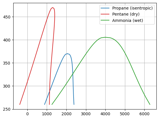
Fig. 25 Illustration of the classification of different heat pump working fluids.

We can make the entropy analysis for each of the three fluids:

fig, ax = plt.subplots(2, sharex=True)

for fluid, data in fluids.items():

    nwk = simple_heat_pump(fluid)
    results = entropy_analysis_temperature_variation(nwk, temperature_range)

    ax[0].plot(temperature_range, results["COP_carnot"], color=data["color"], label=fluid)
    ax[0].plot(temperature_range, results["COP"], "--", color=data["color"])

    ax[1].plot(temperature_range, results["COP"] / results["COP_carnot"], color=data["color"])

ax[1].set_xlabel("Evaporation temperature in °C")

ax[0].set_ylabel("COP")
ax[1].set_ylabel("Efficiency factor")

ax[0].legend()

_ = [_.grid() for _ in ax]
_ = [_.set_axisbelow(True) for _ in ax]

plt.close()

FutureWarning: The API for the component HeatExchangerSimple will change with the next major release, please import SimpleHeatExchanger instead.

FutureWarning: The API for the component HeatExchangerSimple will change with the next major release, please import SimpleHeatExchanger instead.

FutureWarning: The API for the component HeatExchangerSimple will change with the next major release, please import SimpleHeatExchanger instead.

The efficiency factors for the individual working fluids are displayed in Fig. 26. The dry and the isentropic working fluids have increasing efficiency factors, the wet working fluid has a slightly decreasing efficiency factor.

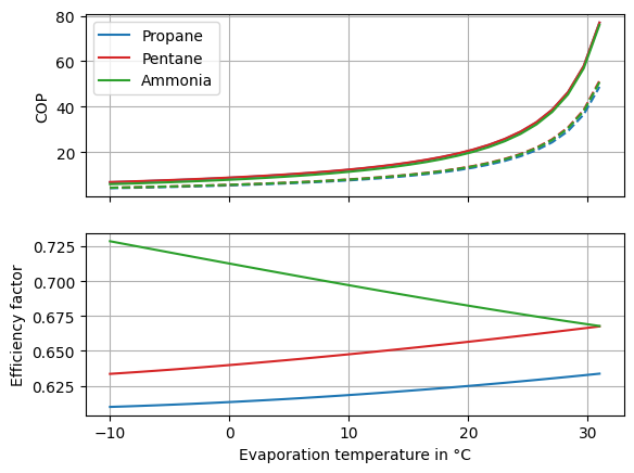
Fig. 26 Efficiency factors of heat pumps using different working fluids.

---

[1]

There is another, more well known, method for the thermodynamic analysis, i.e. the exergy analysis. The method has been implemented in TESPy [6], but since we want to show the connection to the Carnot COP in this excursion, the entropy method is applied.