Linear oemof-solph heat pump model#
In the first section we will implement a heat pump with the Carnot COP method and a linear efficiency factor. For that
we are going to build the system shown in Fig. 3 using oemof-solph.
Build the model#
General setup#
First we are building the components of the system. We do that, by importing the library and create the Bus components
and the electricity grid connection first.
import oemof.solph as solph


b_electricity = solph.Bus(label="electricity")
b_heat_35C = solph.Bus(label="heat 35C")

electricity_grid = solph.components.Source(
    label="electricity grid",
    outputs={b_electricity: solph.Flow(variable_costs=0.4)},  # €/kWh
)
Storage#
Next we add our storage to the system. The storage is connected to the heat bus and has a specified loss rate of 2 %. The nominal capacity of the storage will be 8.7 kWh.
thermal_storage = solph.components.GenericStorage(
    label='thermal storage',
    inputs={b_heat_35C: solph.Flow()},
    outputs={b_heat_35C: solph.Flow()},
    loss_rate=0.02,
    nominal_storage_capacity=8.7,  # Assume 5 k of spread and 1.5 m³ volume
)
Heat demand#
For our heat demand we need a timeseries. We have prepared the data and can load them with a predefined function in this tutorial.
from utilities import load_input_data


input_data = load_input_data().head(24*2)
demand = input_data["Heat load (kW)"][:-1]

demand
2023-01-01 00:00:00    0.00
2023-01-01 01:00:00    0.00
2023-01-01 02:00:00    0.15
2023-01-01 03:00:00    0.20
2023-01-01 04:00:00    0.30
2023-01-01 05:00:00    0.45
2023-01-01 06:00:00    0.50
2023-01-01 07:00:00    0.70
2023-01-01 08:00:00    1.00
2023-01-01 09:00:00    1.15
2023-01-01 10:00:00    1.10
2023-01-01 11:00:00    1.00
2023-01-01 12:00:00    1.00
2023-01-01 13:00:00    0.95
2023-01-01 14:00:00    0.90
2023-01-01 15:00:00    1.10
2023-01-01 16:00:00    1.85
2023-01-01 17:00:00    2.10
2023-01-01 18:00:00    2.15
2023-01-01 19:00:00    2.05
2023-01-01 20:00:00    1.95
2023-01-01 21:00:00    1.25
2023-01-01 22:00:00    0.80
2023-01-01 23:00:00    0.45
2023-01-02 00:00:00    0.25
2023-01-02 01:00:00    0.45
2023-01-02 02:00:00    0.70
2023-01-02 03:00:00    1.00
2023-01-02 04:00:00    1.20
2023-01-02 05:00:00    1.35
2023-01-02 06:00:00    1.65
2023-01-02 07:00:00    1.85
2023-01-02 08:00:00    2.00
2023-01-02 09:00:00    2.25
2023-01-02 10:00:00    2.50
2023-01-02 11:00:00    2.60
2023-01-02 12:00:00    2.75
2023-01-02 13:00:00    2.90
2023-01-02 14:00:00    3.00
2023-01-02 15:00:00    3.05
2023-01-02 16:00:00    3.05
2023-01-02 17:00:00    3.05
2023-01-02 18:00:00    3.15
2023-01-02 19:00:00    3.30
2023-01-02 20:00:00    3.40
2023-01-02 21:00:00    3.60
2023-01-02 22:00:00    3.60
Name: Heat load (kW), dtype: float64
That demand time series can be connected to a Sink component.
heat_demand = solph.components.Sink(
    label="heat demand",
    inputs={b_heat_35C: solph.Flow(nominal_value=1, fix=demand)},  # kW
)
Heat Pump#
Now, we want to add an air-source heat-pump. From a quick research we find the following example [8]:
Rated heating output (kW) at operating point A7/W35: 9.1 kW
Coefficient of performance COP A7/W35: 4.9
From the datasheet we know what the COP of the heat pump is for a specific set of temperatures at nominal load, i.e.
an ambient temperature of 7 °C and
heat production temperature of 35 °C.
However, we do not know, the COP at ambient temperature levels different from 7 °C. With the efficiency factor from eq. (5) and the definition of the Carnot COP (eq. (4)) we can find the actual COP of the heat pump under the assumption, that the efficiency factor is a constant value. We can plot the data
datasheet_cop = 4.9

carnot_cop_7_35 = (35+273.15) / (35-7)
cpf_7_35 = datasheet_cop / carnot_cop_7_35

input_data["cpf COP 7 -> 35"] = cpf_7_35 * (35+273.15) / (35 - input_data["Ambient temperature (°C)"])
However, note that we have to use the maximum and minimum temperature of the process when working with the Carnot COP. The figure Fig. 4 shows two different representations of the heat pump: One as a black box and one as component based process. In the black box process, we only see the temperature levels of the air and the water system. In the actual heat pump heat is transferred from the air to the working fluid and from the working fluid to the water system. This cannot happen without thermodynamic losses, meaning that the temperature of the working fluid must be lower than the air temperature when evaporating and the temperature must be higher when condensing and providing heat to the water system. This however changes our reference temperature levels for the Carnot COP, as the maximum and minimum temperatures of the process are not the air and water temperatures but refer to the working fluid.

Fig. 4 Heat pump black box compared to actual heat pump process#
Since we do not have any internal data of the heat pump, we have to make an assumption to determine the Carnot COP in this way. For both heat exchangers we assume a temperature difference of 5 K, therefore a condensation temperature of 40 °C and an evaporation temperature of 2 °C. This changes our Carnot COP, and given, that we want to have the same COP as in our first assessment, the efficiency factor.
import numpy as np

carnot_cop_2_40 = (40+273.15) / (40-2)
cpf_2_40 = datasheet_cop / carnot_cop_2_40

input_data["cpf COP 2 -> 40"] = cpf_2_40 * (40 + 273.15) / (40 - input_data["Ambient temperature (°C)"] + 5)


temperature_range = np.arange(-10, 21)
cop_7_35 = cpf_7_35 * (35 + 273.15) / (35 - temperature_range)
cop_2_40 = cpf_2_40 * (40 + 273.15) / (40 - temperature_range + 5)
Caution
Due to the reference supply temperature this specific calculation only makes sense in the context of ambient temperature values below 35 °C or evaporation temperature value of 40 °C respectively, because it is only meant for a heat sink temperature of those values. If you want to look at the operation at higher source temperature levels, or at different heat sink temperature levels, you need to adjust the values in the formula respectively.
We can have a look at the difference between both approaches in Fig. 5. The left subplot shows the COP with both approaches over a range of the ambient temperature between -10 and 20 °C. There we can see, that both methods yield the same outcome for 7 °C, i.e. 4.9. For higher temperatures the variant with 7/35 as reference temperatures is higher, for the lower temperatures the variant with 2/40 as reference temperatures has a higher COP. The right subplot shows the COP time series for our application example. Since the ambient temperature is mostly higher than 7 °C, the implementation of the 7/35 variant will have higher COP most of the time.
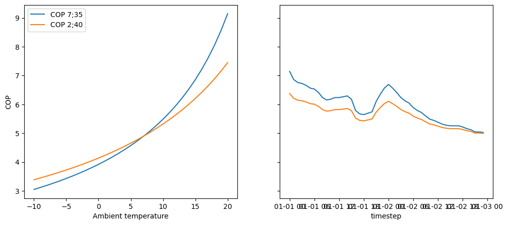
Fig. 5 Comparison of the COP of the heat pump calculated with 7/35 and 2/40 as reference temperature values.#
import matplotlib.pyplot as plt


fig, ax  = plt.subplots(1, 2, sharey=True, figsize=(12, 5))

ax[0].plot(temperature_range, cop_7_35, label="COP 7;35")
ax[0].plot(temperature_range, cop_2_40, label="COP 2;40")

ax[0].set_ylabel("COP")
ax[0].set_xlabel("Ambient temperature")

ax[1].plot(input_data["cpf COP 7 -> 35"])
ax[1].plot(input_data["cpf COP 2 -> 40"])

ax[0].legend()

_ = ax[1].set_xlabel("timestep")

plt.close()
With this information we can create the heat pump, we will use the 2/40 temperature reference.
hp_thermal_power = 9.1  # kW

cop = input_data["cpf COP 2 -> 40"][:-1]
heat_pump = solph.components.Converter(
    label="heat pump",
    inputs={b_electricity: solph.Flow()},
    outputs={b_heat_35C: solph.Flow(nominal_value=hp_thermal_power)},
    conversion_factors={
        b_electricity: 1 / cop,
        b_heat_35C: 1,
    },
)
Optimize the energy system#
Finally, with all components in place we can create the energy system, add the components and run the optimization.
es = solph.EnergySystem(timeindex=input_data.index, infer_last_interval=False)

es.add(b_electricity, b_heat_35C)
es.add(electricity_grid, heat_demand)
es.add(heat_pump)
es.add(thermal_storage)

model = solph.Model(energysystem=es)
model.solve()
results = solph.processing.results(model)
FutureWarning: Series.__getitem__ treating keys as positions is deprecated. In a future version, integer keys will always be treated as labels (consistent with DataFrame behavior). To access a value by position, use `ser.iloc[pos]`
FutureWarning: Series.__getitem__ treating keys as positions is deprecated. In a future version, integer keys will always be treated as labels (consistent with DataFrame behavior). To access a value by position, use `ser.iloc[pos]`
FutureWarning: Series.__getitem__ treating keys as positions is deprecated. In a future version, integer keys will always be treated as labels (consistent with DataFrame behavior). To access a value by position, use `ser.iloc[pos]`
After running the optimization we extract the results and create a figure for the duration curve of the heat pump operation and the demand time series as well as the dispatch of the heat pump and the storage. Fig. 6 shows the results of our first simple implementation. The heat pump is mostly operated in a way to provide the heat demand directly without using the storage as the storage losses make that option unattractive. Only in a single time step the heat pump feeds additional heat to the storage to make use of a advantageous COP for the production of the heat. A total of 14.09 kWh of electricity is consumed.
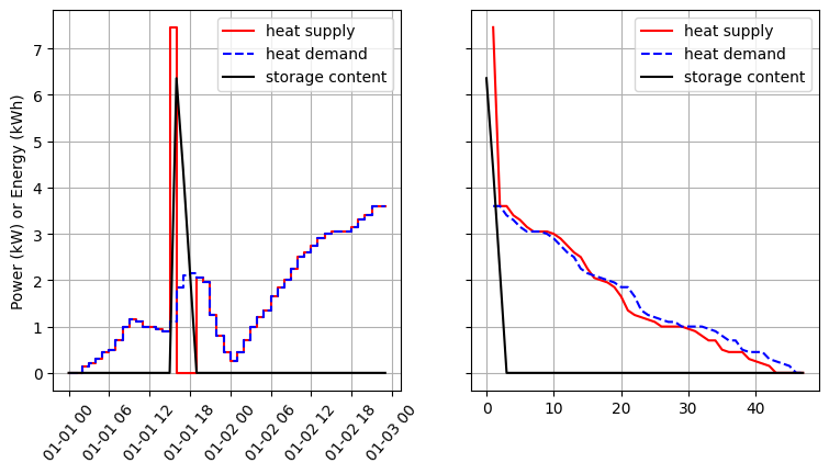
Fig. 6 Results of the simple heat pump setup.#
Tip
We have included a function sumarise_solph_results, which extracts the dispatch of the heat pump, the demand and the
storage filling level to create comparable plots in all sections.
def sumarise_solph_results(results):
    results = solph.views.convert_keys_to_strings(results)

    heat_supply = results[("heat pump", "heat 35C")]["sequences"]["flow"]
    storage_content = results[("thermal storage", "None")]["sequences"]["storage_content"]
    demand = results[("heat 35C", "heat demand")]["sequences"]["flow"]

    fig, (ax1, ax2) = plt.subplots(1, 2, sharey=True, figsize=(9, 4.5))

    ax1.plot(heat_supply, "r-", label="heat supply", drawstyle="steps-post")
    ax1.plot(demand, "b--", label="heat demand", drawstyle="steps-post")
    ax1.plot(storage_content, "k-", label="storage content")
    ax1.set_ylabel("Power (kW) or Energy (kWh)")
    ax1.tick_params(axis="x", rotation=50)
    ax1.grid()
    ax1.legend()

    ax2.plot(np.sort(heat_supply)[::-1], "r-", label="heat supply")
    ax2.plot(np.sort(demand)[::-1], "b--", label="heat demand")
    ax2.plot(np.sort(storage_content)[::-1], "k-", label="storage content")
    ax2.grid()
    ax2.legend()

    electricity_consumption = float(results[("electricity grid", "electricity")]["sequences"]["flow"].sum())
    print(f"Electricity demand: {electricity_consumption:.1f} kWh")
    return fig, electricity_consumption
from utilities import sumarise_solph_results

fig, electricity_total = sumarise_solph_results(results)
plt.close()
Electricity demand: 14.1 kWh