oemof-solph model with variable partload efficiency

The final modification in our energy system model is to implement the load dependent variable COP. To do that we can use the OffsetConverter. This component requires different input compared to our previous implementations. Instead of a conversion factor connecting input with output as shown in eq. (8), we define a slope \(m\) and a normed offset \(E_0\). By setting the reference to the heat output of the heat pump, the compressor power can be determined from the slope and the offset following eq. (9). This also changes the overall efficiency value in an interesting way per eq. 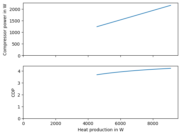(10): We have nonlinear efficiency in a linear model. We can visualize the effect in Fig. 20. For that we load the TESPy results and plot the compressor power and COP over the heat production.

(8)\[\dot E_\text{in} = \frac{1}{\text{COP}} \cdot \dot E_\text{out}\]

(9)\[\dot E_\text{in} = E_0 \cdot \dot E_\text{out,nominal} + m \cdot \dot E_\text{out}\]

(10)\[\text{COP} = \frac{\dot E_\text{out}}{E_0 \cdot \dot E_\text{out,nominal} + m \cdot \dot E_\text{out}}\]

Fig. 20 Compressor power and COP as function of the heat pump heat production at 7 °C.

from utilities import load_tespy_coefficients, load_input_data
from matplotlib import pyplot as plt
import numpy as np


input_data = load_input_data().head(24*2)
tespy_coefficients = load_tespy_coefficients()

example = tespy_coefficients.loc[7]

heat_nominal = 9.1e3
heat_production_range = np.linspace(0.5, 1) * heat_nominal
compressor_power = example.loc["offset"] * heat_nominal + example.loc["slope"] * heat_production_range
cop = heat_production_range / compressor_power

fig, ax = plt.subplots(2, sharex=True)

ax[0].plot(heat_production_range, compressor_power)
ax[0].set_ylim([0, compressor_power.max() * 1.05])
ax[0].set_ylabel("Compressor power in W")

ax[1].plot(heat_production_range, cop)
ax[1].set_ylim([0, cop.max() * 1.05])
ax[1].set_ylabel("COP")

ax[1].set_xlabel("Heat production in W")
ax[1].set_xlim([0, heat_production_range.max() * 1.05])

plt.close()

We can transform the input data from the TESPy model by mapping them onto the ambient temperatures similarly as we had done this for the linear model.

input_data["slope"] = input_data["Ambient temperature (d°C)"].map(tespy_coefficients["slope"])
input_data["offset"] = input_data["Ambient temperature (d°C)"].map(tespy_coefficients["offset"])

Then we load the energy system and add the heat pump with the necessary changes:

from utilities import create_energy_system_stub

es, bus_electricity, bus_heat_35C = create_energy_system_stub(input_data)

With respect to the previous version using minimal load), the Converter is replaced by an OffsetConverter.

import oemof.solph as solph

hp_thermal_power = heat_nominal / 1e3  # kW

slope = input_data["slope"][:-1]
offset = input_data["offset"][:-1]
demand = input_data["Heat load (kW)"][:-1]


heat_pump = solph.components.OffsetConverter(
        label=f"heat pump",
        inputs={bus_electricity: solph.Flow()},
        outputs={
            bus_heat_35C: solph.Flow(
                nominal_value=hp_thermal_power,
                nonconvex=solph.NonConvex(),
                min=0.5,
            )
        },
        conversion_factors={bus_electricity: slope},
        normed_offsets={bus_electricity: offset}
)

es.add(heat_pump)

We can solve our model and have a look at the results.

model = solph.Model(energysystem=es)
model.solve()
results = solph.processing.results(model)

FutureWarning: Series.__getitem__ treating keys as positions is deprecated. In a future version, integer keys will always be treated as labels (consistent with DataFrame behavior). To access a value by position, use `ser.iloc[pos]`

FutureWarning: Series.__getitem__ treating keys as positions is deprecated. In a future version, integer keys will always be treated as labels (consistent with DataFrame behavior). To access a value by position, use `ser.iloc[pos]`

FutureWarning: Series.__getitem__ treating keys as positions is deprecated. In a future version, integer keys will always be treated as labels (consistent with DataFrame behavior). To access a value by position, use `ser.iloc[pos]`

FutureWarning: Series.__getitem__ treating keys as positions is deprecated. In a future version, integer keys will always be treated as labels (consistent with DataFrame behavior). To access a value by position, use `ser.iloc[pos]`

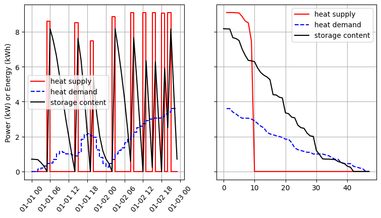
In our final example Fig. 21 shows that the heat pump is mostly operated at full load. This is because the COP of the heat pump in largest in that point (see Fig. 20). The storage losses are higher overall as the filling level is higher as well. However, the increased storage losses are lower than those induced by decrease of the heat pump’s COP in part load. The overall electricity consumption consequently increases from 14.23 kWh to 14.29 kWh.

Fig. 21 Operation of the heat pump modeled as OffsetConverter.

from utilities import sumarise_solph_results

fig, electricity_total = sumarise_solph_results(results)
plt.close()

Electricity demand: 14.3 kWh