Disection of the partload efficiency

Disection of the partload efficiency#

In this section we will provide some more insights on the part load modeling of the individual components of the heat pump. For this we are looking in the characteristics for

compressor efficiency,
evaporator heat transfer coefficient and
condenser heat transfer coefficient.

We investigate the heat load influence at the design point ambient temperature for all cases as this has a stronger effect than the temperature dependency as show in the section on the part load efficiency modeling.

First, we can import the partload_heat_pump function from the provided python script and create a network.

Tip

The partload_heat_pump function imported in this section lies in a separate python document. You can download it: heat_pump_models.py.

from heat_pump_models import partload_heat_pump
from heat_pump_models import AMBIENT_TEMP_NOMINAL, HEAT_NOMINAL


import pandas as pd
import numpy as np
from matplotlib import pyplot as plt


nwk = partload_heat_pump("R290")
nwk.save("R290-design-state")

Next we create a design simulation as reference for all part load simulations.

heat_range = np.linspace(0.5, 1.0, 11) * HEAT_NOMINAL
results_heat = pd.DataFrame(
    index=heat_range,
    columns=["compressor-power", "pressure-ratio", "COP"]
)

cd, cp, ev = nwk.get_comp(["condenser", "compressor", "evaporator"])
c11, c12 = nwk.get_conn(["11", "12"])

c11.set_attr(T=AMBIENT_TEMP_NOMINAL)

for heat in heat_range[::-1]:
    cd.set_attr(Q=heat)
    nwk.solve("design")

    results_heat.loc[heat, "compressor-power"] = cp.P.val
    results_heat.loc[heat, "pressure-ratio"] = cp.pr.val
    results_heat.loc[heat, "COP"] = abs(cd.Q.val) / cp.P.val

Effect of compressor efficiency#

Now we can investigate the compressor efficiency effect on the part load operation. For that, we set up the part load modeling assumptions and test the implementation.

cd.set_attr(Q=HEAT_NOMINAL)
cp.set_attr(design=["eta_s"], offdesign=["eta_s_char"])
cp.eta_s_char.char_func.extrapolate = True

# check if the model runs
nwk.solve("offdesign", design_path="R290-design-state")

Then we can loop over the heat load range and calculate respective results.

results_heat_partload = pd.DataFrame(
    index=heat_range,
    columns=["compressor-power", "pressure-ratio", "COP"]
)

for heat in heat_range[::-1]:
    cd.set_attr(Q=heat)
    nwk.solve("offdesign", design_path="R290-design-state")

    results_heat_partload.loc[heat, "compressor-power"] = cp.P.val
    results_heat_partload.loc[heat, "pressure-ratio"] = cp.pr.val
    results_heat_partload.loc[heat, "COP"] = abs(cd.Q.val) / cp.P.val

Finally, we plot the results. We can see, that the pressure ratio does not depend on the compressor’s efficiency. Still, the COP drops with decreased heat load. The reason for that is the lower part load efficiency of the compressor.

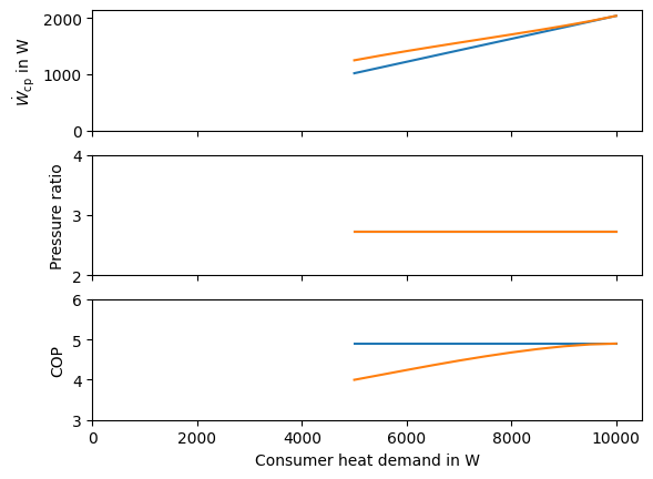
../_images/2c84352057a199c980aaafa97d6e8f872d0e06819f453aa93bc92aefc2dafd13.png — Fig. 27 Influence of the compressor efficiency part load model with varying heat load.#

fig, ax = plt.subplots(3, sharex=True)

ax[0].plot(np.abs(heat_range), results_heat["compressor-power"], label="no partload")
ax[1].plot(np.abs(heat_range), results_heat["pressure-ratio"])
ax[2].plot(np.abs(heat_range), results_heat["COP"])
ax[0].plot(np.abs(heat_range), results_heat_partload["compressor-power"], label="partload")
ax[1].plot(np.abs(heat_range), results_heat_partload["pressure-ratio"])
ax[2].plot(np.abs(heat_range), results_heat_partload["COP"])

ax[0].set_ylabel("$\dot W_\\mathrm{cp}$ in W")
ax[1].set_ylabel("Pressure ratio")
ax[2].set_ylabel("COP")

ax[0].set_ylim([0, results_heat["compressor-power"].max() * 1.05])
ax[1].set_ylim([2, 4])
ax[2].set_ylim([3, 6])
ax[2].set_xlim([0, np.abs(heat_range).max() * 1.05])

_ = ax[2].set_xlabel("Consumer heat demand in W")

plt.close()

Effect of evaporator heat transfer coefficient#

Next, we have a look at the evaporator. We reset the heat demand to the nominal demand, unset the compressor efficiency characteristic to make it use the constant design efficiency and apply the characteristic for the heat transfer coefficient of the evaporator. Then we loop over the heat range again and plot the results.

cd.set_attr(Q=HEAT_NOMINAL)
cp.set_attr(design=[], offdesign=[], eta_s=cp.eta_s.design, eta_s_char=None)
ev.set_attr(design=["ttd_u"], offdesign=["kA_char"])

# check if the model runs
nwk.solve("offdesign", design_path="R290-design-state")

Datacontainer of type ComponentCharacteristics has no attribute "is_var".

results_heat_partload = pd.DataFrame(
    index=heat_range,
    columns=["compressor-power", "pressure-ratio", "COP"]
)

for heat in heat_range[::-1]:
    cd.set_attr(Q=heat)
    nwk.solve("offdesign", design_path="R290-design-state")

    results_heat_partload.loc[heat, "compressor-power"] = cp.P.val
    results_heat_partload.loc[heat, "pressure-ratio"] = cp.pr.val
    results_heat_partload.loc[heat, "COP"] = abs(cd.Q.val) / cp.P.val

In the plot we can see, that the increases at decreasing heat load. The reason for that lies in the reduced pressure ratio, which means that the compressor has to provide less power for compressing the same mass flow. The reduced pressure ratio is finally a result of the heat transfer at the evaporator: If less heat is transferred on the evaporator while the heat transfer coefficient remains more or less unchanged, the available surface for heat transfer allows for lower temperature difference. Since the ambient temperature level is fixed, the evaporation temperature rises compared to the design case reducing the pressure ratio inside the main cycle of the heat pump.

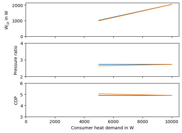
../_images/2cff3829953115eae088cd122a8ddedff5605991d1ab583beb5967ce7226d44e.png — Fig. 28 Influence of the evaporator heat transfer coefficient part load model with varying heat load.#

fig, ax = plt.subplots(3, sharex=True)

ax[0].plot(np.abs(heat_range), results_heat["compressor-power"], label="no partload")
ax[1].plot(np.abs(heat_range), results_heat["pressure-ratio"])
ax[2].plot(np.abs(heat_range), results_heat["COP"])

ax[0].plot(np.abs(heat_range), results_heat_partload["compressor-power"], label="partload")
ax[1].plot(np.abs(heat_range), results_heat_partload["pressure-ratio"])
ax[2].plot(np.abs(heat_range), results_heat_partload["COP"])

ax[0].set_ylabel("$\dot W_\\mathrm{cp}$ in W")
ax[1].set_ylabel("Pressure ratio")
ax[2].set_ylabel("COP")

ax[0].set_ylim([0, results_heat["compressor-power"].max() * 1.05])
ax[1].set_ylim([2, 4])
ax[2].set_ylim([3, 6])
ax[2].set_xlim([0, np.abs(heat_range).max() * 1.05])

_ = ax[2].set_xlabel("Consumer heat demand in W")

plt.close()

Effect of condenser heat transfer coefficient#

Last we investigate the effect of the heat transfer coefficient of the condenser with the analogous setup as for the evaporator.

cd.set_attr(Q=HEAT_NOMINAL)
ev.set_attr(design=[], offdesign=[], ttd_l=ev.ttd_l.design, kA_char=None)
cd.set_attr(design=["ttd_u"], offdesign=["kA_char"])

# check if the model runs
nwk.solve("offdesign", design_path="R290-design-state")

Datacontainer of type GroupedComponentCharacteristics has no attribute "is_var".

results_heat_partload = pd.DataFrame(
    index=heat_range,
    columns=["compressor-power", "pressure-ratio", "COP"]
)

for heat in heat_range[::-1]:
    cd.set_attr(Q=heat)
    nwk.solve("offdesign", design_path="R290-design-state")

    results_heat_partload.loc[heat, "compressor-power"] = cp.P.val
    results_heat_partload.loc[heat, "pressure-ratio"] = cp.pr.val
    results_heat_partload.loc[heat, "COP"] = abs(cd.Q.val) / cp.P.val

In the plot we can see an even stronger relationship between the decrease of heat load and the decrease of pressure ratio, therefore the increase in COP. The effect is the same as we have observed in the evaporator.

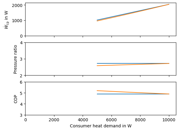
../_images/8bc3abd61a1feb722eb75015e06766d2e80a9e32dec39fa978ee3c49c7af0280.png — Fig. 29 Influence of the condenser heat transfer coefficient part load model with varying heat load.#

fig, ax = plt.subplots(3, sharex=True)

ax[0].plot(np.abs(heat_range), results_heat["compressor-power"], label="no partload")
ax[1].plot(np.abs(heat_range), results_heat["pressure-ratio"])
ax[2].plot(np.abs(heat_range), results_heat["COP"])
ax[0].plot(np.abs(heat_range), results_heat_partload["compressor-power"], label="partload")
ax[1].plot(np.abs(heat_range), results_heat_partload["pressure-ratio"])
ax[2].plot(np.abs(heat_range), results_heat_partload["COP"])

ax[0].set_ylabel("$\dot W_\\mathrm{cp}$ in W")
ax[1].set_ylabel("Pressure ratio")
ax[2].set_ylabel("COP")

ax[0].set_ylim([0, results_heat["compressor-power"].max() * 1.05])
ax[1].set_ylim([2, 4])
ax[2].set_ylim([3, 6])
ax[2].set_xlim([0, np.abs(heat_range).max() * 1.05])

_ = ax[2].set_xlabel("Consumer heat demand in W")

plt.close()