Combining oemof-solph and TESPy

After running the TESPy model to determine the COP at different ambient temperature values, the next steps are as follows:

• read the results from the TESPy model,

• make an interpolation to map the results to the actual ambient temperature time series and

• pass the COP time series to the heat pump in the oemof-solph model.

Note

The oemof-solph model will have the identical components as in the previous model. The only change is, that we use a different source for our COP time series. We will therefore import a ready to use oemof-solph EnergySysten from our utilities script to save some space here and only add the heat pump.

from utilities import load_input_data, create_energy_system_stub
input_data = load_input_data().head(24*2)

es, bus_electricity, bus_heat_35C = create_energy_system_stub(input_data)

FutureWarning: The 'delim_whitespace' keyword in pd.read_csv is deprecated and will be removed in a future version. Use ``sep='\s+'`` instead

Build the heat pump model

To build the heat pump model we load the COP from the TESPy simulation first and then map the ambient temperature data from our ambient temperature time series to the TESPy lookup data.

from utilities import load_tespy_cop

tespy_cop = load_tespy_cop()
tespy_cop

	COP
temperature
-100.0	3.327825
-99.0	3.334274
-98.0	3.340723
-97.0	3.347171
-96.0	3.353620
...	...
306.0	7.577904
307.0	7.577904
308.0	7.577904
309.0	7.577904
310.0	7.577904

411 rows × 1 columns

We can compare the TESPy COP with the datasheet and constant efficiency factor approach in Fig. 9. They are, as expected, very similar.

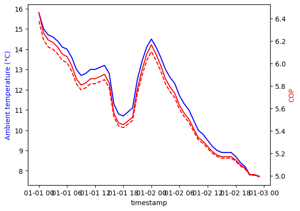
Fig. 9 Comparison of the COP time series from the constant efficiency method with the TESPy model.

input_data["simple TESPy COP"] = input_data["Ambient temperature (d°C)"].map(tespy_cop["COP"])


datasheet_cop = 4.9
carnot_cop_2_40 = (40+273.15) / (40-2)
cpf_2_40 = datasheet_cop / carnot_cop_2_40

input_data["cpf COP 2 -> 40"] = cpf_2_40 * (40 + 273.15) / (40 - input_data["Ambient temperature (°C)"] + 5)


from matplotlib import pyplot as plt


fig, ax = plt.subplots(1)

ax.plot(input_data["Ambient temperature (d°C)"]/10, "b-")
ax.set_ylabel("Ambient temperature (°C)").set_color("blue")
ax.set_xlabel("timestamp")

ax2 = ax.twinx()

ax2.plot(input_data["simple TESPy COP"], "r-")
ax2.plot(input_data["cpf COP 2 -> 40"], "r--")
ax2.set_ylabel("COP").set_color("red")

plt.close()

import oemof.solph as solph


hp_thermal_power = 9.1  # kW
cop = input_data["simple TESPy COP"][:-1]

heat_pump = solph.components.Converter(
    label="heat pump",
    inputs={bus_electricity: solph.Flow()},
    outputs={bus_heat_35C: solph.Flow(nominal_value=hp_thermal_power)},
    conversion_factors={
        bus_electricity: 1 / cop,
        bus_heat_35C: 1,
    },
)

es.add(heat_pump)

Run the model

Finally, we can run our optimization model and read the results again.

model = solph.Model(energysystem=es)
model.solve()
results = solph.processing.results(model)

FutureWarning: Series.__getitem__ treating keys as positions is deprecated. In a future version, integer keys will always be treated as labels (consistent with DataFrame behavior). To access a value by position, use `ser.iloc[pos]`

FutureWarning: Series.__getitem__ treating keys as positions is deprecated. In a future version, integer keys will always be treated as labels (consistent with DataFrame behavior). To access a value by position, use `ser.iloc[pos]`

FutureWarning: Series.__getitem__ treating keys as positions is deprecated. In a future version, integer keys will always be treated as labels (consistent with DataFrame behavior). To access a value by position, use `ser.iloc[pos]`

FutureWarning: Series.__getitem__ treating keys as positions is deprecated. In a future version, integer keys will always be treated as labels (consistent with DataFrame behavior). To access a value by position, use `ser.iloc[pos]`

Fig. 10 shows nearly identical behavior as in the simple setup. Only the electricity consumption changed very slightly from 14.09 kWh to 14.03 kWh.

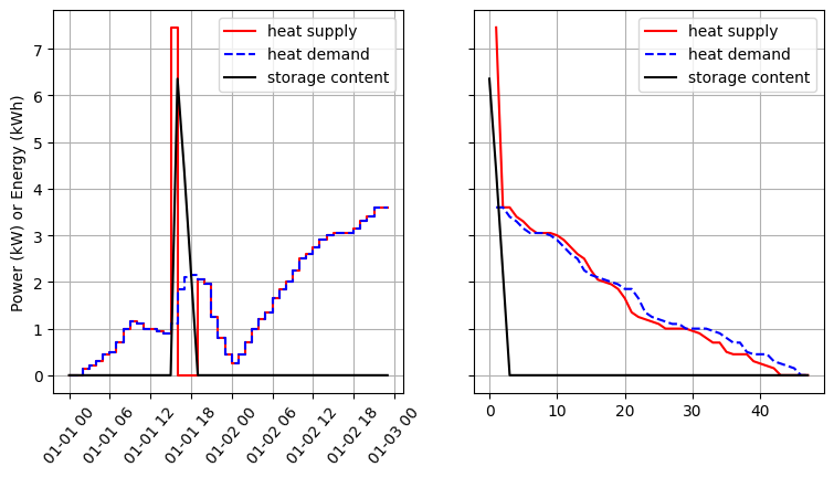
Fig. 10 Results of the simple heat pump setup using the COP data from TESPy.

from utilities import sumarise_solph_results

fig, electricity_total = sumarise_solph_results(results)
plt.close()

WARNING:TESPyLogger:FutureWarning: Calling float on a single element Series is deprecated and will raise a TypeError in the future. Use float(ser.iloc[0]) instead

Electricity demand: 14.0 kWh